FUZZEKS [to Index]
Quick start: Fuzzy kriging
The typical procedure for working with FUZZEKS
This page describes (with help of a very simple example) how to
1. prepare a data file,
2. load the data file,
3. prepare the fuzzy kriging process (and perform fuzzy kriging) and
4. view and export the fuzzy kriging result.
If you are additionally interested in aggregating parameters, you
should go through this page first and then read about
1. Preparing a data file
The ASCII input data file consists of a sequence of the following sections:
- A "region" section (the bottom left, bottom right and
top left corner of the area where fuzzy kriging should be performed),
e.g.:
region
    0    0
 1800    0
    0 1800
- A "cuts" section.
Determination of the representation of fuzzy data in the form of
fuzzy numbers.
In FUZZEKS fuzzy numbers are represented by so-called level-cuts
(for FUZZEKS intervals of values where the membership
function value is greater the level (or equal the level if the level is 1)).
As example the cuts section
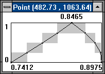
"cuts 1 0.75 0.5 0.25 0" leads to a representation of the
fuzzy numbers with 5 level-cuts as can also be seen in the display of
the membership function for such a fuzzy number:

At least you have to choose the levels 1 and 0 as in the following example:
cuts
    1    0
- A "parameters" section (a list of the parameters in this file, each
of them occupies a single line), e.g.:
parameters
    Cl_concentration
- A "table" section (contains the data itself, Cl_concentration
entries explained below), e.g.:
table
  X    Y   Cl_concentration

 165 1630    20
 460 1690    30
 435 1500    40
 105 1265    40
 300 1080    75
 560 1240    80/0:50-130
1010 1600    65
1400 1600    85
1350 1260   130
1510  950   175
1710  650   150
 540  530   145/0:95-195
 225  755    90
  70  590    70
 210  130    65
 435  130   100
 930   45   105/0:55-155
1010  275   160
1135  175   130
1185  360   170
1705  415   125
1625  160    85
 915 1270   101
1000 1165   130
 860 1100   130
1770 1545    85
1135 1070   155
 705  870   145
1190  750   220
1055  545   210
The entry 80/0:50-130 means the value is most possibly 80, but it can not
be smaller than 50 or greater than 130 (which is the simplest representation
of a fuzzy number in FUZZEKS and which corresponds to the levels 1 and 0 -
if more levels of cuts have been defined in the cuts section, the other
level-cuts would be interpolated (linear)).
- And at last the word end.
More detailed information at
"FDF inputfile format".
2. Loading the data file
After saving this textual information as ASCII data file (e.g.
"TEST.FDF"), press F3 (or select "Load input file"
from the "Project" menu) and then select this file.
As only visible result of loading an input data file (as e.g. the file
that consists of the example sections above), the following contents in the
management window will appear.

3. Preparing the fuzzy kriging process (and perform fuzzy kriging)
Click at the small window icon ( ) of the left box (see the
management window's contents above) in order to open
a "Kriging window":

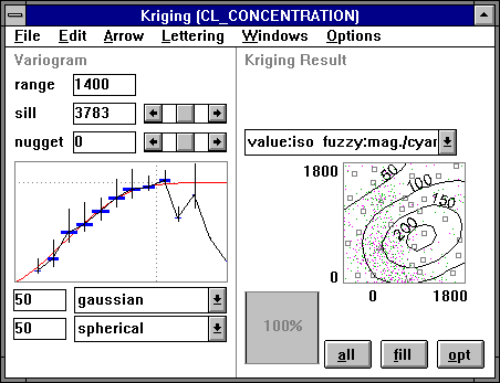
The left part of the window contains the display of the
experimental variogram and the theoretical variogram.
The theoretical variogram's parameters can be seen
in the input fields and listboxes.
The right part of the window shows the kriging result, the corresponding
listbox of display methods and some buttons to control the visible area.
The meaning of the variogram is explained in
Kriging Basics / Theoretical concepts. A description of the variogram
graphics is found in Handling Variograms.
The facilities to diplay the kriging result are described in
Result Display Options.
The preparation of the fuzzy kriging process must be done in two steps:
- Setting of the experimental variogram's calculation options.
- Selection of a theoretical variogram that fits the experimental variogram.
The window will look a bit different to the above picture at first. You
must prepare the experimental variogram (by the dialog window
"Options"/"Experimental_Variogram") and enter the
correct values in the input-fields at the left ("variogram") side of the
window.
(For the example presented above the calculation option
"Number of groups" in the dialog window
"Options"/"Experimental_Variogram" has been set to 9.)
Of course, the settings depend on the actual input data.
To find a proper theoretical variogram (a variogram function - described by
the parameters in the edit and listbox fields - that fits the experimental
variogram) should be done with care, because its quality determines
the quality of the kriging results.
A detailed description for fitting the theoretical variogram can be found
on the page Theoretical variogram fitting
(Function types and parameters).
If you do not use the above example data you must fix a different theoretical
variogram, of course.
For simple testing purposes, where the quality of the kriging result is not
important, a 100% linear theoretical variogram should do (instead of this
50% gaussian and 50% spherical theoretical variogram in the above example).
This variogram type has the advantage that the kriging result is independant
of range, sill and nugget effect, so the values of these parameters are
always sufficient.
As warning there must be said that it is not a common variogram type,
it is only easy to handle!
You need not to start the kriging process; it is started automatically
everytime when a recalculation is needed, which guarantees that all
displayed information in the kriging window fits together anytime
(the status of the calculations can be seen at the top of the screen).
4. Viewing and exporting the fuzzy kriging result
In order to get a meaningful display as shown above, some options must be
changed in the dialog window "Options"/"Isolines/Dither"
(in this example a difference of values between isolines of 50 and a
dither factor of 10 has been chosen).
The size of the result graphics (at the right side) can be changed by the
buttons at the bottom right of the window (the "all"-button usually
should change it to a good size).
The lettering of the isolines can be achieved by dragging an arrow in the
display with the mouse and then pressing "L" (at the intersections
of isolines with the arrow an inscription is placed). The dialog window
"Options"/"Lettering" can change the format and size of the
numbers.
After following the above instructions
the display shows isolines for the most possible values
(in this case, with respect to these isolines, there is no difference between
the usual crisp and fuzzy kriging results). The data points are small squares
for crisp input values and small triangles for the fuzzy values (and small
"u"s indicate undefined values (positions where other parameters
have a value or where an "undef" has been assigned in the input
data file)). The fuzziness of the result (possible deviations of the results)
is displayed as density of the small dots. More detailed
information at
Result basics / Overview and
Result Display Options / Overview, where
other types of result-display are also described.
The graphical result can be exported to the clipboard by selecting
"Edit"/"Copy result to clipboard", an ASCII representation
can be obtained
by "File"/"Krige values for raster and save to ascii-file", which
needs an additional inputfile, described at
Export of results
.


 ) of the left box (see the
management window's contents above) in order to open
a "Kriging window":